神經網路識別手寫（Mnist）

神經網路識別手寫（Mnist）

前言

本文是之前我們實現的神經網路對手寫體識別的一個實踐。使用的數據是經典的Mnist數據。
下載鏈接爲：
http://www.iro.umontreal.ca/~lisa/deep/data/mnist/mnist.pkl.gz

官網地址是http://yann.lecun.com/exdb/mnist/

數據讀取

這裏直接使用別人提供的讀取函數。

# -*- coding: utf-8 -*-
# @Time    : 2017/11/24 上午10:27
# @Author  : SkullFang
# @Email   : [email protected]
# @File    : mnist_loader.py
# @Software: PyCharm
"""
mnist_loader
~~~~~~~~~~~~

A library to load the MNIST image data.  For details of the data
structures that are returned, see the doc strings for ``load_data``
and ``load_data_wrapper``.  In practice, ``load_data_wrapper`` is the
function usually called by our neural network code.
"""

#### Libraries
# Standard library
import cPickle
import gzip

# Third-party libraries
import numpy as np

def load_data():
    """Return the MNIST data as a tuple containing the training data,
    the validation data, and the test data.

    The ``training_data`` is returned as a tuple with two entries.
    The first entry contains the actual training images.  This is a
    numpy ndarray with 50,000 entries.  Each entry is, in turn, a
    numpy ndarray with 784 values, representing the 28 * 28 = 784
    pixels in a single MNIST image.

    The second entry in the ``training_data`` tuple is a numpy ndarray
    containing 50,000 entries.  Those entries are just the digit
    values (0...9) for the corresponding images contained in the first
    entry of the tuple.

    The ``validation_data`` and ``test_data`` are similar, except
    each contains only 10,000 images.

    This is a nice data format, but for use in neural networks it's
    helpful to modify the format of the ``training_data`` a little.
    That's done in the wrapper function ``load_data_wrapper()``, see
    below.
    """
    f = gzip.open('../data/mnist.pkl.gz', 'rb')
    training_data, validation_data, test_data = cPickle.load(f)
    f.close()
    return (training_data, validation_data, test_data)

def load_data_wrapper():
    """Return a tuple containing ``(training_data, validation_data,
    test_data)``. Based on ``load_data``, but the format is more
    convenient for use in our implementation of neural networks.

    In particular, ``training_data`` is a list containing 50,000
    2-tuples ``(x, y)``.  ``x`` is a 784-dimensional numpy.ndarray
    containing the input image.  ``y`` is a 10-dimensional
    numpy.ndarray representing the unit vector corresponding to the
    correct digit for ``x``.

    ``validation_data`` and ``test_data`` are lists containing 10,000
    2-tuples ``(x, y)``.  In each case, ``x`` is a 784-dimensional
    numpy.ndarry containing the input image, and ``y`` is the
    corresponding classification, i.e., the digit values (integers)
    corresponding to ``x``.

    Obviously, this means we're using slightly different formats for
    the training data and the validation / test data.  These formats
    turn out to be the most convenient for use in our neural network
    code."""
    tr_d, va_d, te_d = load_data()
    training_inputs = [np.reshape(x, (784, 1)) for x in tr_d[0]]
    training_results = [vectorized_result(y) for y in tr_d[1]]
    training_data = zip(training_inputs, training_results)
    validation_inputs = [np.reshape(x, (784, 1)) for x in va_d[0]]
    validation_data = zip(validation_inputs, va_d[1])
    test_inputs = [np.reshape(x, (784, 1)) for x in te_d[0]]
    test_data = zip(test_inputs, te_d[1])
    return (training_data, validation_data, test_data)

def vectorized_result(j):
    """Return a 10-dimensional unit vector with a 1.0 in the jth
    position and zeroes elsewhere.  This is used to convert a digit
    (0...9) into a corresponding desired output from the neural
    network."""
    e = np.zeros((10, 1))
    e[j] = 1.0
    return e

def load_data_wrapper2():
    """Return a tuple containing ``(training_data, validation_data,
    test_data)``. Based on ``load_data``, but the format is more
    convenient for use in our implementation of neural networks.

    In particular, ``training_data`` is a list containing 50,000
    2-tuples ``(x, y)``.  ``x`` is a 784-dimensional numpy.ndarray
    containing the input image.  ``y`` is a 10-dimensional
    numpy.ndarray representing the unit vector corresponding to the
    correct digit for ``x``.

    ``validation_data`` and ``test_data`` are lists containing 10,000
    2-tuples ``(x, y)``.  In each case, ``x`` is a 784-dimensional
    numpy.ndarry containing the input image, and ``y`` is the
    corresponding classification, i.e., the digit values (integers)
    corresponding to ``x``.

    Obviously, this means we're using slightly different formats for
    the training data and the validation / test data.  These formats
    turn out to be the most convenient for use in our neural network
    code."""
    tr_d, va_d, te_d = load_data()
    training_inputs = [np.reshape(x, (784, 1)) for x in tr_d[0]]
    training_results = [vectorized_result(y) for y in tr_d[1]]
    training_data = zip(training_inputs, training_results)
    validation_inputs = [np.reshape(x, (784, 1)) for x in va_d[0]]
    validation_data = zip(validation_inputs, va_d[1])
    test_inputs = [np.reshape(x, (784, 1)) for x in te_d[0]]
    test_data = zip(test_inputs, te_d[1])
    return (training_inputs, training_results, validation_data, test_data)

數據集分析

數據集其實上面已經寫的很清楚了。我們import之後直接調用即可。

import mnist_loader

       traning_data, validation_data, test_data = mnist_loader.load_data_wrapper()

輸入數據

輸入數據是一個28*28的圖片，還有一個標籤。

首先看輸入x
![這裏寫圖片描述](https://img-blog.csdn.net/20171127185751185?watermark/2/text/aHR0cDovL2Jsb2cuY3Nkbi5uZXQvc2t1bGxGYW5n/font/5a6L5L2T/fontsize/400/fill/I0JBQkFCMA==/dissolve/70/gravity/SouthEast)
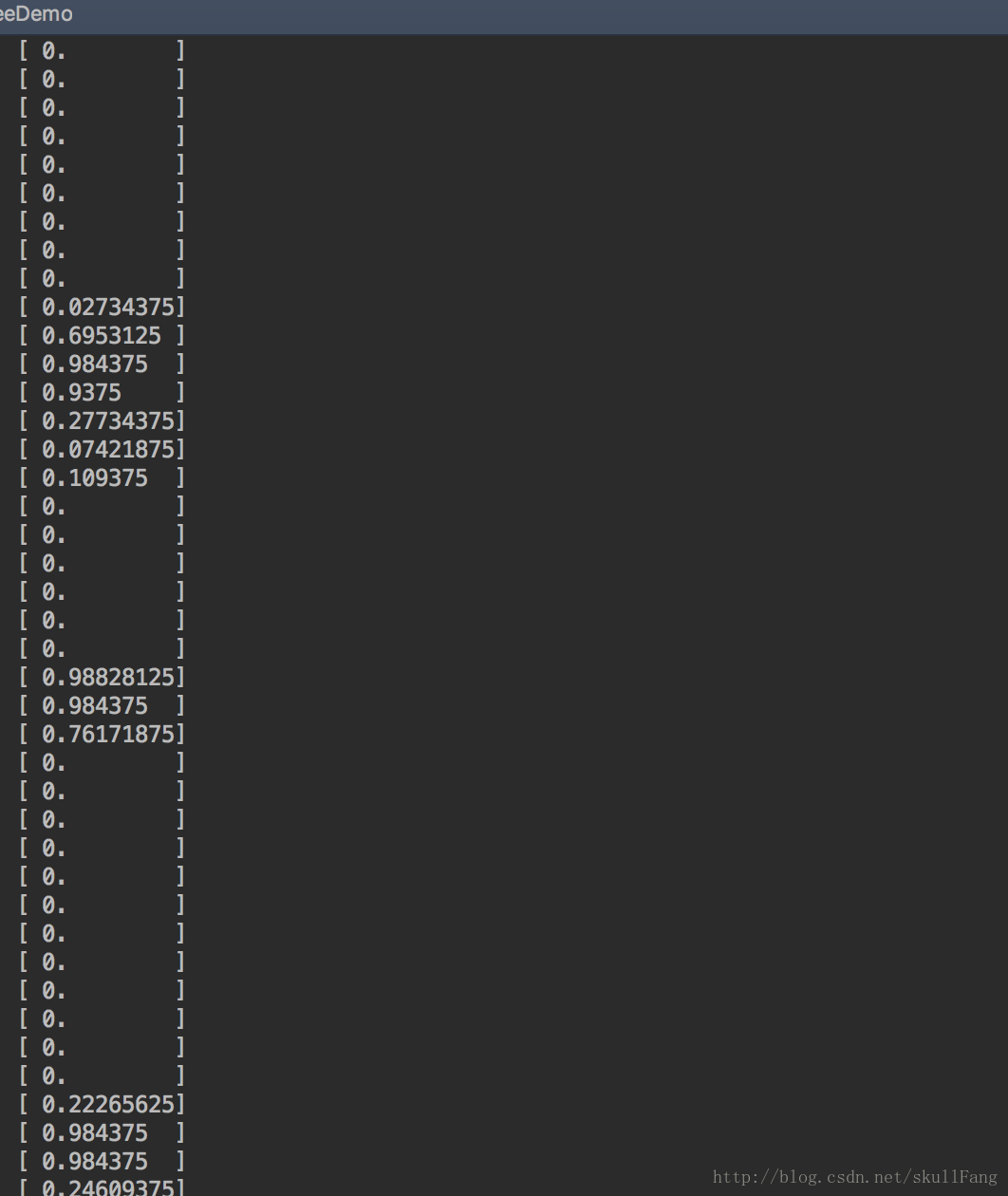
這是片段，我們很容易看出其實每個像素點都是一個輸入。共有28*28=784個輸入。
所以我們的**輸入層**一定是**784個**神經元。一個神經元對應一個輸入。

然後看標籤y
![這裏寫圖片描述](https://img-blog.csdn.net/20171127190027045?watermark/2/text/aHR0cDovL2Jsb2cuY3Nkbi5uZXQvc2t1bGxGYW5n/font/5a6L5L2T/fontsize/400/fill/I0JBQkFCMA==/dissolve/70/gravity/SouthEast)

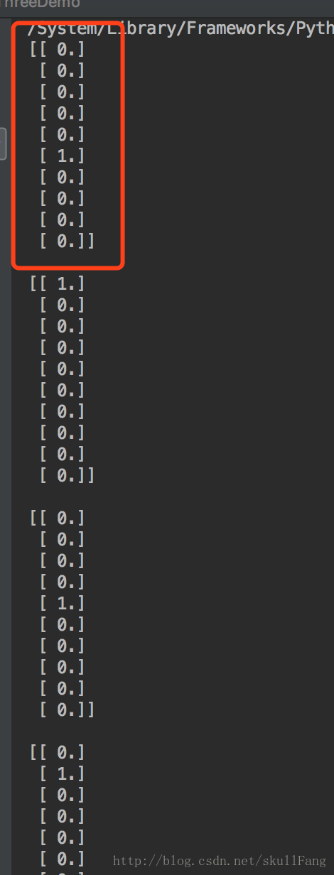
這一組代表一個標籤，我們可以看出，是一個10維的向量。其中只有一個1。說明這是個維度分別代表0、1、2、3、4、5、6、7、8、9。如果哪個維度是1就說明這個是屬於哪個數字。例如上圖對應的應該就是5。

所以我們的輸出層應該是**10個神經元**分別輸出是個數字，其中最大的那個數字就是最有可能的預測。

**隱藏層隨意編寫...**

<h1>隨機梯度下降</h1>
在真的訓練模型的時候需要說一下隨機梯度下降的算法。爲什麼要介紹這個呢？
如果我們直接用梯度下降的話。因爲每次訓練要算出所有維的w,b然後進行計算更新，這個計算量是十分龐大的。如果維度太大，並且一定要使用sigmod激勵函數的話。還有可能導致。
```python
RuntimeWarning: overflow encountered in exp
  return 1.0/(1.0+np.exp(-z))




<div class="se-preview-section-delimiter"></div>

這是一個比較嚴重的問題。於是就有了隨機梯度下降，其實隨機梯度下降思路很簡單。

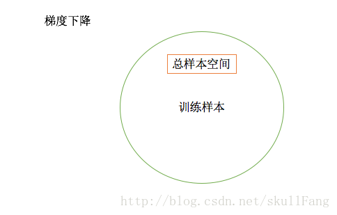
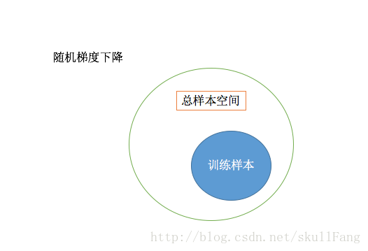
梯度下降每次會計算出所有的訓練樣本從而更新w和b。而隨機梯度下降會每次從訓練樣本中抽取部分進行訓練更新w,b。如圖。

隨機梯度下降

如圖隨機梯度下降在每一輪學習的時候只會隨機挑選總樣本空間的一部分進行訓練。這一部分就是一個batch size。

隨機梯度下降沒有什麼新的東西，其實就是 犧牲精度換效率

代碼部分

在前面的基礎上我們在隨機梯度下降函數中加入一個參數mini_batch。另外更新的時候要用eta除以minibatch的長度（因爲是要更新一個minibatch，而不是所有）
“`

這是一個比較嚴重的問題。於是就有了隨機梯度下降，其實隨機梯度下降思路很簡單。

梯度下降每次會計算出所有的訓練樣本從而更新w和b。而隨機梯度下降會每次從訓練樣本中抽取部分進行訓練更新w,b。如圖。
![這裏寫圖片描述](https://img-blog.csdn.net/20171127191412305?watermark/2/text/aHR0cDovL2Jsb2cuY3Nkbi5uZXQvc2t1bGxGYW5n/font/5a6L5L2T/fontsize/400/fill/I0JBQkFCMA==/dissolve/70/gravity/SouthEast)
隨機梯度下降
![這裏寫圖片描述](https://img-blog.csdn.net/20171127191521179?watermark/2/text/aHR0cDovL2Jsb2cuY3Nkbi5uZXQvc2t1bGxGYW5n/font/5a6L5L2T/fontsize/400/fill/I0JBQkFCMA==/dissolve/70/gravity/SouthEast)

如圖隨機梯度下降在每一輪學習的時候只會隨機挑選總樣本空間的一部分進行訓練。這一部分就是一個batch size。

隨機梯度下降沒有什麼新的東西，其實就是 **犧牲精度換效率**

<h1>代碼部分</h1>
在前面的基礎上我們在隨機梯度下降函數中加入一個參數mini_batch。另外更新的時候要用eta除以minibatch的長度（因爲是要更新一個minibatch，而不是所有）
```python




<div class="se-preview-section-delimiter"></div>

# -*- coding: utf-8 -*-
import random

import numpy as np


class Network(object):
    def __init__(self, sizes):
        # 網絡層數
        self.num_layers = len(sizes)
        # 網絡每層神經元個數
        self.sizes = sizes
        # 初始化每層的偏置
        self.biases = [np.random.randn(y, 1) for y in sizes[1:]]
        # 初始化每層的權重
        self.weights = [np.random.randn(y, x)
                        for x, y in zip(sizes[:-1], sizes[1:])]

    def feedforward(self, a):
        """
        前向傳播 就是計算每個輸入產生的結果
        :param a: 
        :return: 
        """
        for b, w in zip(self.biases, self.weights):
            a = sigmoid(np.dot(w, a) + b)
        return a

    # 隨機梯度下降
    def SGD(self, training_data, epochs, mini_batch_size, eta,
            test_data=None):
        """
        隨機梯度想講
        :param training_data: 
        :param epochs: 
        :param mini_batch_size: 等分成幾份
        :param eta: 
        :param test_data: 
        :return: 
        """
        if test_data: n_test = len(test_data)
        # 訓練數據總個數
        n = len(training_data)

        # 開始訓練 循環每一個epochs
        for j in xrange(epochs):
            # 打亂訓練數據
            random.shuffle(training_data)

            # mini_batch
            #把數據集按照mini_batch大小等分。
            mini_batches = [training_data[k:k + mini_batch_size]
                            for k in range(0, n, mini_batch_size)]


            # 訓練mini_batch，每次訓練的不再是總的而是mini_batch個
            for mini_batch in mini_batches:
                self.update_mini_batch(mini_batch, eta)

            if test_data:
                print "Epoch {0}: {1} / {2}".format(
                    j, self.evaluate(test_data), n_test)
            print "Epoch {0} complete".format(j)

    # 更新mini_batch
    def update_mini_batch(self, mini_batch, eta):
        """
        更新權重和偏置
        :param mini_batch: 
        :param eta: 
        :return: 
        """
        # 保存每層偏倒
        nabla_b = [np.zeros(b.shape) for b in self.biases]
        nabla_w = [np.zeros(w.shape) for w in self.weights]

        # 訓練每一個mini_batch
        for x, y in mini_batch:
            delta_nable_b, delta_nabla_w = self.update(x, y)

            # 保存一次訓練網絡中每層的偏倒
            nabla_b = [nb + dnb for nb, dnb in zip(nabla_b, delta_nable_b)]
            nabla_w = [nw + dnw for nw, dnw in zip(nabla_w, delta_nabla_w)]
        #訓練完了之後就更新，注意這裏更新要處以len(mini_batch)
        # 更新權重和偏置 Wn+1 = wn - eta/len(mini_batch) * nw
        self.weights = [w - (eta / len(mini_batch)) * nw
                        for w, nw in zip(self.weights, nabla_w)]
        self.biases = [b - (eta / len(mini_batch)) * nb
                       for b, nb in zip(self.biases, nabla_b)]


    # 前向傳播和反向傳播
    def update(self, x, y):
        """
        算出更新的偏導
        :param x: 
        :param y: 
        :return: 
        """
        # 保存每層偏導
        nabla_b = [np.zeros(b.shape) for b in self.biases]
        nabla_w = [np.zeros(w.shape) for w in self.weights]

        activation = x

        # 保存每一層的激勵值a=sigmoid(z)
        activations = [x]

        # 保存每一層的z=wx+b
        zs = []
        # 前向傳播
        for b, w in zip(self.biases, self.weights):
            # 計算每層的z
            z = np.dot(w, activation) + b

            # 保存每層的z
            zs.append(z)

            # 計算每層的a
            activation = sigmoid(z)

            # 保存每一層的a
            activations.append(activation)

        # 反向傳播
        # 計算最後一層的誤差
        delta = self.cost_derivative(activations[-1], y) * sigmoid_prime(zs[-1])

        # 最後一層權重和偏置的倒數
        nabla_b[-1] = delta
        nabla_w[-1] = np.dot(delta, activations[-2].transpose())

        # 倒數第二層一直到第一層 權重和偏置的倒數
        for l in range(2, self.num_layers):
            z = zs[-l]

            sp = sigmoid_prime(z)

            # 當前層的誤差
            delta = np.dot(self.weights[-l+1].transpose(), delta) * sp

            # 當前層偏置和權重的倒數
            nabla_b[-l] = delta
            nabla_w[-l] = np.dot(delta, activations[-l - 1].transpose())

        return (nabla_b, nabla_w)

    def evaluate(self, test_data):
        """
        計算一下正確的個數
        :param test_data: 
        :return: 
        """
        test_results = [(np.argmax(self.feedforward(x)), y)
                        for (x, y) in test_data]
        return sum(int(x == y) for (x, y) in test_results)

    def cost_derivative(self, output_activation, y):
        """
        計算輸出和真是值的偏差
        :param output_activation: 
        :param y: 
        :return: 
        """
        return (output_activation - y)


def sigmoid(z):
    """
    激勵函數
    :param z: 
    :return: 
    """
    return 1.0 / (1.0 + np.exp(-z))


def sigmoid_prime(z):
    """
    激勵函數的導數
    :param z: 
    :return: 
    """
    return sigmoid(z) * (1 - sigmoid(z))


if __name__ == '__main__':
    from ProjectOne import mnist_loader

    traning_data, validation_data, test_data = mnist_loader.load_data_wrapper()

    net = Network([784, 30,20, 10])
    net.SGD(traning_data, 30, 10, 0.5, test_data=test_data)





<div class="se-preview-section-delimiter"></div>

我的網絡是三層，輸入層不算。隱藏層兩層，輸出層一層。

  net = Network([784, 30,20, 10])
    net.SGD(traning_data, 30, 10, 0.5, test_data=test_data)

我的網絡是三層，輸入層不算。隱藏層兩層，輸出層一層。
```python
  net = Network([784, 30,20, 10])
    net.SGD(traning_data, 30, 10, 0.5, test_data=test_data)




<div class="se-preview-section-delimiter"></div>

訓練的結果並不是很好
“`

訓練的結果並不是很好

Epoch 0: 8274 / 10000
Epoch 0 complete
Epoch 1: 8759 / 10000
Epoch 1 complete
Epoch 2: 8956 / 10000
Epoch 2 complete
Epoch 3: 9041 / 10000
Epoch 3 complete
Epoch 4: 9094 / 10000
Epoch 4 complete
Epoch 5: 9140 / 10000
Epoch 5 complete
Epoch 6: 9187 / 10000
Epoch 6 complete
Epoch 7: 9208 / 10000
Epoch 7 complete
Epoch 8: 9235 / 10000
Epoch 8 complete
Epoch 9: 9246 / 10000
Epoch 9 complete
Epoch 10: 9247 / 10000
Epoch 10 complete
Epoch 11: 9280 / 10000
Epoch 11 complete
Epoch 12: 9271 / 10000
Epoch 12 complete
Epoch 13: 9290 / 10000
Epoch 13 complete
Epoch 14: 9293 / 10000
Epoch 14 complete
Epoch 15: 9313 / 10000
Epoch 15 complete
Epoch 16: 9320 / 10000
Epoch 16 complete
Epoch 17: 9316 / 10000
Epoch 17 complete
Epoch 18: 9328 / 10000
Epoch 18 complete
Epoch 19: 9312 / 10000
Epoch 19 complete
Epoch 20: 9332 / 10000
Epoch 20 complete
Epoch 21: 9337 / 10000
Epoch 21 complete
Epoch 22: 9366 / 10000
Epoch 22 complete
Epoch 23: 9354 / 10000
Epoch 23 complete
Epoch 24: 9358 / 10000
Epoch 24 complete
Epoch 25: 9364 / 10000
Epoch 25 complete
Epoch 26: 9369 / 10000
Epoch 26 complete
Epoch 27: 9370 / 10000
Epoch 27 complete
Epoch 28: 9376 / 10000
Epoch 28 complete
Epoch 29: 9374 / 10000
Epoch 29 complete
“`

其中還有很大的改進空間。