[深度學習] 自然語言處理 --- 基於Attention機制的Bi-LSTM文本分類

Peng Zhou等發表在ACL2016的一篇論文《Attention-Based Bidirectional Long Short-Term Memory Networks for Relation Classification》。

論文主要介紹了在關係分類任務中應用雙向LSTM神經網絡模型並加入Attention機制，從而避免了傳統工作中複雜的特徵工程，並在該任務中取得比較優秀的效果。

一研究背景與動機

關係抽取（分類）是自然語言處理中一個重要的任務，也即從自然語言文本中提取兩個實體之間的語義關係。關係抽取屬於信息抽取的一個部分。信息激增的時代，快速、準確獲取關鍵信息的需求也日益激增，相比於傳統的信息檢索，信息抽取能夠快速、準確提取出海量非結構化信息中的結構化知識，它也逐漸成爲搜索引擎發展的方向。而關係抽取同命名實體識別、事件抽取等任務一起，都是信息抽取的一部分或者中間過程，可應用於結構化知識抽取、知識圖譜構建、自動問答系統構建等。

關係抽取從本質上看是一個多分類問題，對於這樣一個問題來說最重要的工作無非特徵的提取和分類模型的選擇。傳統的方法中，大多數研究依賴於一些現有的詞彙資源（例如WordNet）、NLP系統或一些手工提取的特徵。這樣的方法可能導致計算複雜度的增加，並且特徵提取工作本身會耗費大量的時間和精力，特徵提取質量的對於實驗的結果也有很大的影響。因此，這篇論文從這一角度出發，提出一個基於Attention機制的雙向LSTM神經網絡模型進行關係抽取研究，Attention機制能夠自動發現那些對於分類起到關鍵作用的詞，使得這個模型可以從每個句子中捕獲最重要的語義信息，它不依賴於任何外部的知識或者NLP系統。

二、算法模型詳解

其他模型裏Attention結構

Hierarchical Attention Networks for Document Classification
這篇文章主要講述了基於Attention機制實現文本分類

假設我們有很多新聞文檔，這些文檔屬於三類：軍事、體育、娛樂。其中有一個文檔D有L個句子si（i代表s是文檔D的第i個句子），每個句子包含Ti個詞（word），wit代表第i個句子的word,t∈[0,T]

Word Encoder：
①給定一個句子si,例如 The superstar is walking in the street，由下面表示[wi1,wi2,wi3,wi4,wi5,wi6,wi1,wi7]，我們使用一個詞嵌入矩陣W將單詞編碼爲向量

②使用雙向GRU編碼整個句子關於單詞wit的隱含向量：

那麼最終隱含向量爲前向隱含向量和後向隱含向量拼接在一起

Word Attention:
給定一句話，並不是這個句子中所有的單詞對個句子語義起同等大小的“貢獻”，比如上句話“The”,“is”等，這些詞沒有太大作用，因此我們需要使用attention機制來提煉那些比較重要的單詞，通過賦予權重以提高他們的重要性。
①通過一個MLP獲取hit的隱含表示：

②通過一個softmax函數獲取歸一化的權重：

③計算句子向量：
通過每個單詞獲取的hit與對應權重αit乘積，然後獲取獲得句子向量

W與b爲Attention的權重與bias，在實現的時候也要設置attention的size，不過也可以簡單的令它們等於BIRNN的輸出向量的size。

Uw也是需要設置的權重，公式(2)其實也就是對所有Ut*Uw結果的softmax。

Tensorflow: https://github.com/ilivans/tf-rnn-attention/blob/master/attention.py

import tensorflow as tf


def attention(inputs, attention_size, time_major=False, return_alphas=False):
    """
    Attention mechanism layer which reduces RNN/Bi-RNN outputs with Attention vector.

    The idea was proposed in the article by Z. Yang et al., "Hierarchical Attention Networks
     for Document Classification", 2016: http://www.aclweb.org/anthology/N16-1174.
    Variables notation is also inherited from the article

    Args:
        inputs: The Attention inputs.
            Matches outputs of RNN/Bi-RNN layer (not final state):
                In case of RNN, this must be RNN outputs `Tensor`:
                    If time_major == False (default), this must be a tensor of shape:
                        `[batch_size, max_time, cell.output_size]`.
                    If time_major == True, this must be a tensor of shape:
                        `[max_time, batch_size, cell.output_size]`.
                In case of Bidirectional RNN, this must be a tuple (outputs_fw, outputs_bw) containing the forward and
                the backward RNN outputs `Tensor`.
                    If time_major == False (default),
                        outputs_fw is a `Tensor` shaped:
                        `[batch_size, max_time, cell_fw.output_size]`
                        and outputs_bw is a `Tensor` shaped:
                        `[batch_size, max_time, cell_bw.output_size]`.
                    If time_major == True,
                        outputs_fw is a `Tensor` shaped:
                        `[max_time, batch_size, cell_fw.output_size]`
                        and outputs_bw is a `Tensor` shaped:
                        `[max_time, batch_size, cell_bw.output_size]`.
        attention_size: Linear size of the Attention weights.
        time_major: The shape format of the `inputs` Tensors.
            If true, these `Tensors` must be shaped `[max_time, batch_size, depth]`.
            If false, these `Tensors` must be shaped `[batch_size, max_time, depth]`.
            Using `time_major = True` is a bit more efficient because it avoids
            transposes at the beginning and end of the RNN calculation.  However,
            most TensorFlow data is batch-major, so by default this function
            accepts input and emits output in batch-major form.
        return_alphas: Whether to return attention coefficients variable along with layer's output.
            Used for visualization purpose.
    Returns:
        The Attention output `Tensor`.
        In case of RNN, this will be a `Tensor` shaped:
            `[batch_size, cell.output_size]`.
        In case of Bidirectional RNN, this will be a `Tensor` shaped:
            `[batch_size, cell_fw.output_size + cell_bw.output_size]`.
    """

    if isinstance(inputs, tuple):
        # In case of Bi-RNN, concatenate the forward and the backward RNN outputs.
        inputs = tf.concat(inputs, 2)

    if time_major:
        # (T,B,D) => (B,T,D)
        inputs = tf.array_ops.transpose(inputs, [1, 0, 2])

    hidden_size = inputs.shape[2].value  # D value - hidden size of the RNN layer

    # Trainable parameters
    w_omega = tf.Variable(tf.random_normal([hidden_size, attention_size], stddev=0.1))
    b_omega = tf.Variable(tf.random_normal([attention_size], stddev=0.1))
    u_omega = tf.Variable(tf.random_normal([attention_size], stddev=0.1))

    with tf.name_scope('v'):
        # Applying fully connected layer with non-linear activation to each of the B*T timestamps;
        #  the shape of `v` is (B,T,D)*(D,A)=(B,T,A), where A=attention_size
        v = tf.tanh(tf.tensordot(inputs, w_omega, axes=1) + b_omega)

    # For each of the timestamps its vector of size A from `v` is reduced with `u` vector
    vu = tf.tensordot(v, u_omega, axes=1, name='vu')  # (B,T) shape
    alphas = tf.nn.softmax(vu, name='alphas')  # (B,T) shape

    # Output of (Bi-)RNN is reduced with attention vector; the result has (B,D) shape
    output = tf.reduce_sum(inputs * tf.expand_dims(alphas, -1), 1)

    if not return_alphas:
        return output
    else:
        return output, alphas

Pytorch:

class Attention(nn.Module):
    def __init__(self, feature_dim, step_dim, bias=True, **kwargs):
        super(Attention, self).__init__(**kwargs)
        
        self.supports_masking = True

        self.bias = bias
        self.feature_dim = feature_dim
        self.step_dim = step_dim
        self.features_dim = 0
        
        weight = torch.zeros(feature_dim, 1)
        nn.init.kaiming_uniform_(weight)
        self.weight = nn.Parameter(weight)
        
        if bias:
            self.b = nn.Parameter(torch.zeros(step_dim))
        
    def forward(self, x, mask=None):
        feature_dim = self.feature_dim 
        step_dim = self.step_dim

        eij = torch.mm(
            x.contiguous().view(-1, feature_dim), 
            self.weight
        ).view(-1, step_dim)
        
        if self.bias:
            eij = eij + self.b
            
        eij = torch.tanh(eij)
        a = torch.exp(eij)
        
        if mask is not None:
            a = a * mask

        a = a / (torch.sum(a, 1, keepdim=True) + 1e-10)

        weighted_input = x * torch.unsqueeze(a, -1)
        return torch.sum(weighted_input, 1)

論文中模型結構

Bi-LSTM + Attention 就是在Bi-LSTM的模型上加入Attention層，在Bi-LSTM中我們會用最後一個時序的輸出向量作爲特徵向量，然後進行softmax分類。Attention是先計算每個時序的權重，然後將所有時序的向量進行加權和作爲特徵向量，然後進行softmax分類。在實驗中，加上Attention確實對結果有所提升。

輸入層：將句子輸入到模型中
Embedding層：將每個詞映射到低維空間
LSTM層：使用雙向LSTM從Embedding層獲取高級特徵
Attention層：生成一個權重向量，通過與這個權重向量相乘，使每一次迭代中的詞彙級的特徵合併爲句子級的特徵。
輸出層：將句子級的特徵向量用於關係分類

embedding通常有兩種處理方法，一個是靜態embedding，即通過事先訓練好的詞向量，另一種是動態embedding，即伴隨着網絡一起訓練；

2.1 輸入層

輸入層輸入的是以句子爲單位的樣本。

2.2 Word Embeddings

對於一個給定的包含T個詞的句子S: S=x1,x2,…,xT。每一個詞xi都是轉換爲一個實數向量ei。對於S中的每一個詞來說，首先存在一個詞向量矩陣：Wwrd∈ℝdw|V|，其中V是一個固定大小的詞彙表，dw是詞向量的維度，是一個由用戶自定義的超參數，Wwrd則是通過訓練學習到的一個參數矩陣。使用這個詞向量矩陣，可以將每個詞轉化爲其詞向量的表示：其中，vi是一個大小爲|V| 的one-hot向量，在下表爲ei處爲1，其他位置爲0。於是，句子S將被轉化爲一個實數矩陣：$$emb_s = {e_1, e_2, …, e_T}$，並傳遞給模型的下一層。

2.3 Bi-LSTM

LSTM最早由Hochreiter和Schmidhuber (1997)提出，爲了解決循環神經網絡中的梯度消失問題。主要思想是引入門機制，從而能夠控制每一個LSTM單元保留的歷史信息的程度以及記憶當前輸入的信息，保留重要特徵，丟棄不重要的特徵。這篇論文采用了Graves等人(2013)提出的一個變體，將上一個細胞狀態同時引入到輸入門、遺忘門以及新信息的計算當中。對於序列建模的任務來說，每一個時刻的未來信息和歷史信息同等重要，標準的LSTM模型按其順序並不能捕獲未來的信息。

因而這篇論文采用了雙向LSTM模型，在原有的正向LSTM網絡層上增加一層反向的LSTM層，可以表示成：hi=[h⃗ i⨁hi←]

2.4 Attention機制

由於LSTM獲得每個時間點的輸出信息之間的“影響程度”都是一樣的，而在關係分類中，爲了能夠突出部分輸出結果對分類的重要性，引入加權的思想，注意力機制本質上就是加權求和。

將LSTM層輸入的向量集合表示爲H：[h1,h2,…,hT]。其Attention層得到的權重矩陣由下面的方式得到：

其中，H∈ℝdw×T，dw爲詞向量的維度，wT是一個訓練學習得到的參數向量的轉置。最終用以分類的句子將表示如下 :h∗=tanh(r)

Pytorch1

class GRUWithAttention(nn.Module):
    def __init__(self, vocab_size, embedding_dim, n_hidden, n_out, bidirectional=False):
        super().__init__()
        self.vocab_size = vocab_size
        self.embedding_dim = embedding_dim
        self.n_hidden = n_hidden
        self.n_out = n_out
        self.bidirectional = bidirectional

        self.emb = nn.Embedding(self.vocab_size, self.embedding_dim)
        self.emb_drop = nn.Dropout(0.3)
        self.gru = nn.GRU(self.embedding_dim, self.n_hidden, dropout=0.3, bidirectional=bidirectional)
        
        # attention layer
        self.attention_layer = nn.Sequential(
            nn.Linear(self.n_hidden*2, self.n_hidden*2),
            nn.ReLU(inplace=True)
        )
        
        if bidirectional:
            self.fc = nn.Linear(self.n_hidden*2, self.n_out)
        else:
            self.fc = nn.Linear(self.n_hidden, self.n_out)
            
        
    def forward(self, seq, lengths):
        self.h = self.init_hidden(seq.size(1))
        embs = self.emb_drop(self.emb(seq))
        embs = pack_padded_sequence(embs, lengths)
        
        gru_out, self.h = self.gru(embs, self.h)
        gru_out, lengths = pad_packed_sequence(gru_out)  
        gru_out = gru_out.permute(1, 0, 2)
        
        attention_out = self.attention(gru_out)
        outp = self.fc(attention_out)          
        return F.log_softmax(outp, dim=-1) # it will return log of softmax
    
    def init_hidden(self, batch_size):
        # initialized to zero, for hidden state and cell state of LSTM
        number = 1
        if self.bidirectional:
           number = 2
        return torch.zeros((number, batch_size, self.n_hidden), requires_grad=True).to(device)
      
    def attention(self, h):
        m = nn.Tanh()(h)
        # [batch_size, time_step, hidden_dims]
        w = self.attention_layer(h)
        # [batch_size, time_step, time_step]
        alpha = F.softmax(torch.bmm(m, w.transpose(1, 2)), dim=-1)
        
        context = torch.bmm(h.transpose(1,2), alpha) 
        result = nn.Tanh()(torch.sum(context, dim=-1))
        
        return result

Pytorch2

class GRUWithAttention2(nn.Module):
    def __init__(self, vocab_size, embedding_dim, n_hidden, n_out, bidirectional=False):
        super().__init__()
        self.vocab_size = vocab_size
        self.embedding_dim = embedding_dim
        self.n_hidden = n_hidden
        self.n_out = n_out
        self.bidirectional = bidirectional

        self.emb = nn.Embedding(self.vocab_size, self.embedding_dim)
        self.emb_drop = nn.Dropout(0.3)
        self.gru = nn.GRU(self.embedding_dim, self.n_hidden, dropout=0.3, bidirectional=bidirectional)
        
        weight = torch.zeros(1, self.n_hidden*2)
        nn.init.kaiming_uniform_(weight)
        self.attention_weights = nn.Parameter(weight)
                
        if bidirectional:
            self.fc = nn.Linear(self.n_hidden*2, self.n_out)
        else:
            self.fc = nn.Linear(self.n_hidden, self.n_out)
            
        
    def forward(self, seq, lengths):
        self.h = self.init_hidden(seq.size(1))
        embs = self.emb_drop(self.emb(seq))
        embs = pack_padded_sequence(embs, lengths)
        
        gru_out, self.h = self.gru(embs, self.h)
        gru_out, lengths = pad_packed_sequence(gru_out)  
        gru_out = gru_out.permute(1, 0, 2)
        
        attention_out = self.attention(gru_out)
        outp = self.fc(attention_out)          
        return F.log_softmax(outp, dim=-1) # it will return log of softmax
    
    def init_hidden(self, batch_size):
        # initialized to zero, for hidden state and cell state of LSTM
        number = 1
        if self.bidirectional:
           number = 2
        return torch.zeros((number, batch_size, self.n_hidden), requires_grad=True).to(device)
     
    def attention(self, h):
        batch_size = h.size()[0]
        m = F.tanh(h)
        # apply attention layer
        hw = torch.bmm(m, # (batch_size,  time_step, hidden_size*2)
                        self.attention_weights  # (1, hidden_size*2)
                        .permute(1, 0)  # (hidden_size, 1)
                        .unsqueeze(0)  # (1, hidden_size, 1)
                        .repeat(batch_size, 1, 1) # (batch_size, hidden_size*2, 1)
                        )
        
        alpha = F.softmax(hw, dim=-1)
        context = torch.bmm(h.transpose(1,2), alpha)
        result = F.tanh(torch.sum(context, dim=-1))
        return result

Tensorflow參考

    def attention(self, H):
        """
        利用Attention機制得到句子的向量表示
        """
        
        # 對Bi-LSTM的輸出用激活函數做非線性轉換
        M = tf.tanh(H)

        # 獲得最後一層LSTM的神經元數量
        hiddenSize = config.model.hiddenSizes[-1]
        # 初始化一個權重向量，是可訓練的參數
        W = tf.Variable(tf.random_normal([hiddenSize], stddev=0.1))
        # 對W和M做矩陣運算，W=[batch_size, time_step, hidden_size]，計算前做維度轉換成[batch_size * time_step, hidden_size]
        # newM = [batch_size, time_step, 1]，每一個時間步的輸出由向量轉換成一個數字
        newM = tf.matmul(tf.reshape(M, [-1, hiddenSize]), tf.reshape(W, [-1, 1]))
        

        # 對newM做維度轉換成[batch_size, time_step]
        restoreM = tf.reshape(newM, [-1, config.sequenceLength])
        # 用softmax做歸一化處理[batch_size, time_step]
        self.alpha = tf.nn.softmax(restoreM)
        
        # 利用求得的alpha的值對H進行加權求和，用矩陣運算直接操作
        r = tf.matmul(tf.transpose(H, [0, 2, 1]), tf.reshape(self.alpha, [-1, config.sequenceLength, 1]))
        
        # 將三維壓縮成二維sequeezeR=[batch_size, hidden_size]
        sequeezeR = tf.reshape(r, [-1, hiddenSize])
        
        sentenceRepren = tf.tanh(sequeezeR)
        
        # 對Attention的輸出可以做dropout處理
        output = tf.nn.dropout(sentenceRepren, self.dropoutKeepProb)
        
        return output

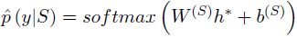
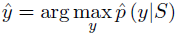
2.5 損失函數

分類使用一個softmax分類器來預測標籤ŷ 。該分類器將上一層得到的隱狀態作爲輸入:

成本函數採用正樣本的負對數似然：

其中t∈ℜm爲正樣本的one-hot表示，y∈ℜm爲softmax估計出的每個類別的概率（m爲類別個數），λ是L2正則化的超參數。這篇論文中使用了Dropout和L2正則化的組合以減輕過擬合的情況。

[深度學習] 自然語言處理 --- 基於Attention機制的Bi-LSTM文本分類

一研究背景與動機

二、算法模型詳解

2.1 輸入層

2.2 Word Embeddings

2.3 Bi-LSTM

2.4 Attention機制

2.5 損失函數

[數據處理] Pandas利用groupby拆分csv

[深度學習] 自然語言處理 --- 文本分類模型總結

[kubernetes] 證書詳細總結

[深度學習]自然語言處理 --- ELMo

[Linux]Centos 6.3 下源代碼安裝gcc 4.8.2/4.9.2

https://yachay.unat.edu.pe/blog/index.php?comment_area=format_blog&comment_component=blog&comment_co

linux以太網驅動總結

[深度學習] 自然語言處理 --- 基於Attention機制的Bi-LSTM文本分類

一 研究背景與動機

二、算法模型詳解

2.1 輸入層

2.2 Word Embeddings

2.3 Bi-LSTM

2.4 Attention機制

2.5 損失函數

一研究背景與動機