


When Ian Goodfellow dreamt up the idea of Generative Adversarial Networks (GANs) over a mug of beer back in 2014, he probably didn’t expect to see the field advance so fast:

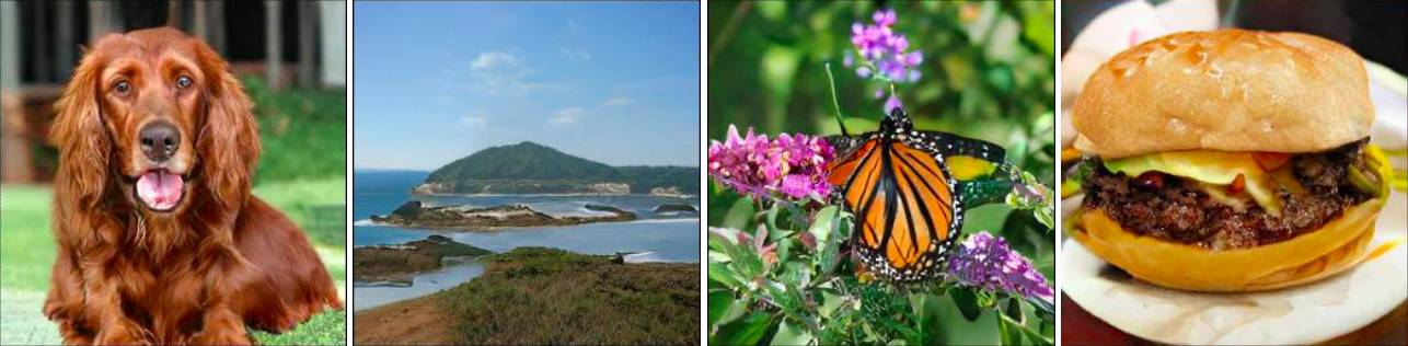
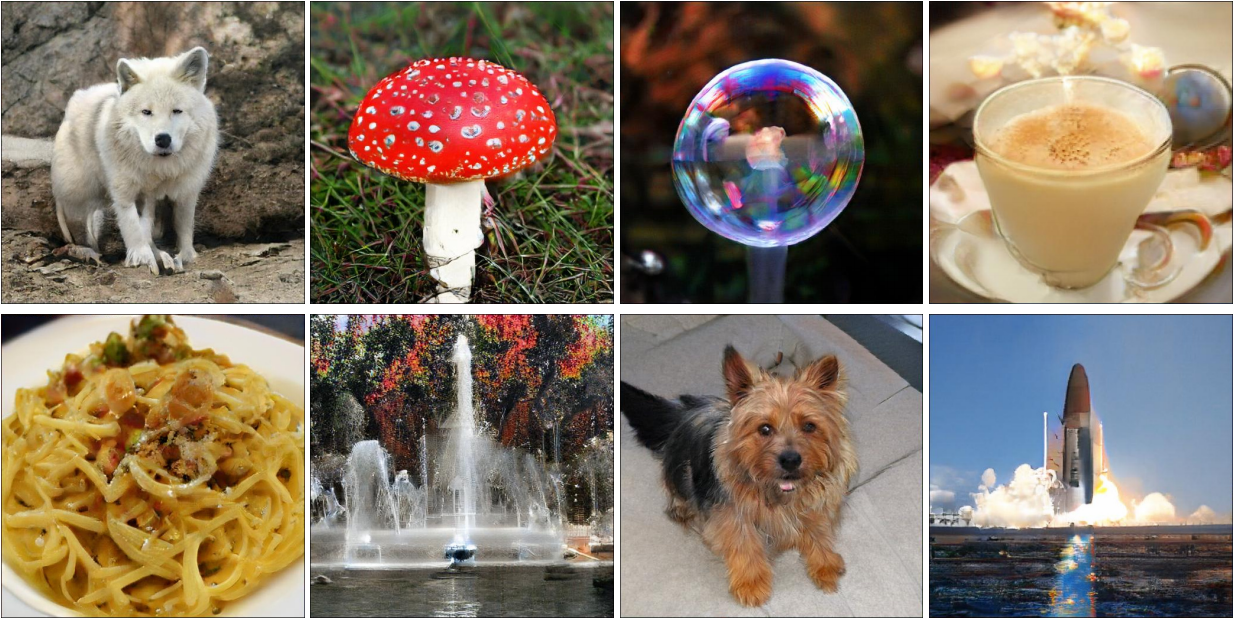
In case you don’t see where I’m going here, the images you just saw were utterly, undeniably, 100% … fake.
Also, I don’t mean these were photoshopped, CGI-ed, or (fill in the blanks with whatever Nvidia’s calling their fancy new tech at the moment).
I mean that these images are entirely generated through addition, multiplication, and splurging ludicrous amounts of cash on GPU computation.
The algorithm that makes is stuff work is called a generative adversarial network (which is the long way of writing GAN, for those of you still stuck in machine learning acronym land), and over the last few years, there have been more innovations dedicated to making it work than there have been privacy scandals at Facebook.
4.5 years of GAN progress on face generation. https://t.co/kiQkuYULMChttps://t.co/S4aBsU536b https://t.co/8di6K6BxVChttps://t.co/UEFhewds2M https://t.co/s6hKQz9gLzpic.twitter.com/F9Dkcfrq8l
— Ian Goodfellow (@goodfellow_ian) January 15, 2019
Summarizing every single improvement to the 2014 vanilla GANs is about as hard as watching season 8 of Game of Thrones on repeat. So instead, I’m going to recap the key ideas behind some of the coolest results in GAN research over the years.
I’m not going to explain concepts like transposed convolutions and Wasserstein distance in detail. Instead, I’ll provide links to some of the best resources you can use to quickly learn about these concepts so that you can see how they fit into the big picture.
If you’re still reading, I’m going to assume that you know the basics of deep learning and that you know how convolutional neural networks work.
With that said, here’s the map of the GAN landscape:

GAN Roadmap
We’ll traverse it one step at a time. Let the journey begin.
- GAN: Generative Adversarial Networks
- DCGAN: Deep Convolutional Generative Adversarial Network
- CGAN: Conditional Generative Adversarial Network
- CycleGAN
- CoGAN: Coupled Generative Adversarial Networks
- ProGAN: Progressive growing of Generative Adversarial Networks
- WGAN: Wasserstein Generative Adversarial Networks
- SAGAN: Self-Attention Generative Adversarial Networks
- BigGAN: Big Generative Adversarial Networks
- StyleGAN: Style-based Generative Adversarial Networks
GAN: Generative Adversarial Networks

Image from paper
- Paper
- Code
- Other great resources: Ian Goodfellow’s NIPS 2016 tutorial
Now, I know what you’re thinking — geez, that creepy, pixelated mess of an image looks like it was made by a math nerd zooming out of an excel sheet.
Well, guess what, you’re somewhat right (minus the excel part).
Way back in 2014, Ian Goodfellow proposed a revolutionary idea — make two neural networks compete (or collaborate, it’s a matter of perspective) with each other.
One neural network tries to generate realistic data (note that GANs can be used to model any data distribution, but are mainly used for images these days), and the other network tries to discriminate between real data and data generated by the generator network.
The generator network uses the discriminator as a loss function and updates its parameters to generate data that starts to look more realistic.

The discriminator network, on the other hand, updates its parameters to make itself better at picking out fake data from real data. So it too gets better at its job.
The game of cat and mouse continues, until the system reaches a so-called “equilibrium,” where the generator creates data that looks real enough that the best the discriminator can do is guess randomly.
Hopefully, by this point, if you indented your code correctly and Amazon decided not to kill your spot instances(by the way, this will not happen on FloydHub since they provide reserved GPU machines), you're now left with a generator that accurately creates new data from the same distribution as your training set.
Now, this is admittedly a very simplistic view of GANs. The idea you need to take away from here is that by using two neural networks - one to generate data and one to classify real data from fake data, you can simultaneously train them to, in theory, converge to a point where the generator can generate completely new, realistic data.
DCGAN: Deep Convolutional Generative Adversarial Network

Image from paper
- Paper
- Code
- Other great resources: Medium article
Look, I’ll save you some time.
[Math Processing Error]Convolutions=Good for images
[Math Processing Error]GANs=Good for generating stuff
[Math Processing Error]⟹Convolutions+GANs=Good for generating images
In hindsight, as Ian Goodfellow himself pointed out in a podcast with Lex Fridman, it seems silly to call this model DCGAN (short for “deep convolutional generative adversarial network”) since almost everything related to deep learning and images these days is deep and convolutional.
Plus, when most people are introduced to GANs, they learn about them in the “deep and convolutional” setting anyway. 🤷
Nevertheless, there existed a time when GANs did not necessarily use convolution-based operation and instead relied upon a standard multi-layer perceptron architecture.
DCGAN changed that by using something called a transposed convolution operation or, its "unfortunate" name, Deconvolution layer,.
Transposed convolutions act as an upscaling operation. They help us transform low-resolution images into higher resolution ones.
But seriously, go through the above resources to nail down your understanding of transposed convolutions, since this operation is fundamental to all modern GAN architectures.
If you’re a little short on time though, an excellent summary of how transposed convolutions work can be found in one simple animation:

In vanilla convnets, you apply a sequence of convolutions (along with other operations) to map an image to a vector that usually lower dimensional.
Similarly, applying multiple transposed convolutions sequentially allows us to evolve a single, low-resolution array into a vibrant, full-color image.
Now before we continue, let’s venture off on a small tangent to explore some unique ways of using GANs.

You're currently at the second red 'X'
CGAN: Conditional Generative Adversarial Network

Image from paper
The original GAN generates data from random noise. That means that you can train it on, say, dog images, and it would generate more dog images.
You could also train it on cat images, in which case, it would generate cat images.
You could also train it on Nicholas Cage images, in which case, it would generate Nicholas Cage images.
You could also train it on… I hope you’re sensing a pattern here.
However, if you try to train it on both dog and cat images at the same time, it’ll produce blurry half-breeds.

Photo by Anusha Barwa on Unsplash
CGAN (which stands for “conditional generative adversarial network”) aims to solve this issue by telling the generator to generate images of only one particular class, like a cat, dog, or Nicholas Cage.
Specifically, CGAN concatenates a one-hot vector [Math Processing Error]y to the random noise vector [Math Processing Error]z to result in an architecture that looks like this:

Now, we can generate both cats and dogs from the very same GAN. 🐈 🐕
CycleGAN

- Paper
- Code
- Other great resources: CycleGAN project page, Medium article
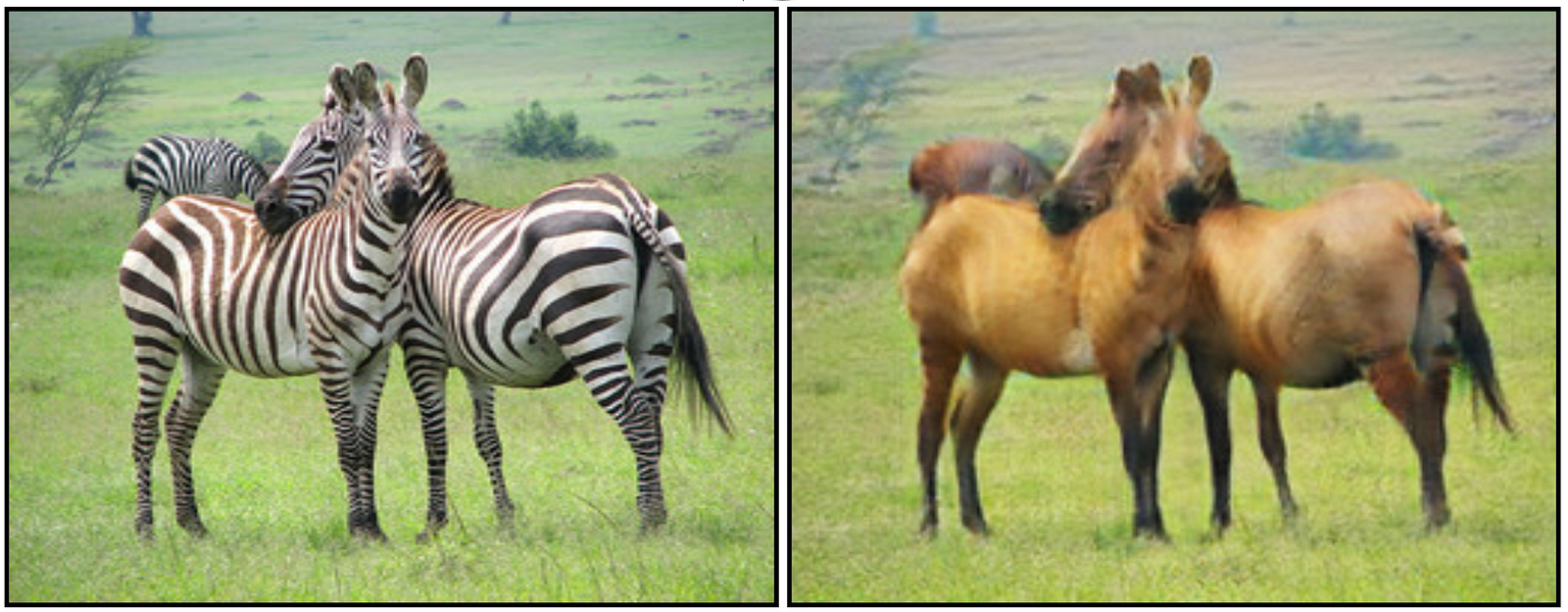
GANs aren’t used just for generating images. They can also create horse+zebra creatures (zorses? hobras?) like in the image above.
To create these images, CycleGAN aims to solve a problem called image-to-image translation.
CycleGAN isn’t a new GAN architecture that pushes the state of the art image synthesis. Instead, it’s a smart way of using GANs. So you’re free to use this technique for any architecture you like.
Right off the bat, I’m going to recommend that you read this paper. It’s exceptionally well written and is quite accessible, even to beginners.
The task here is to train a network [Math Processing Error]G(X) that maps images from a source domain [Math Processing Error]X to a target domain [Math Processing Error]Y.
But wait, “how is this different from regular deep learning or style transfer,” you ask.
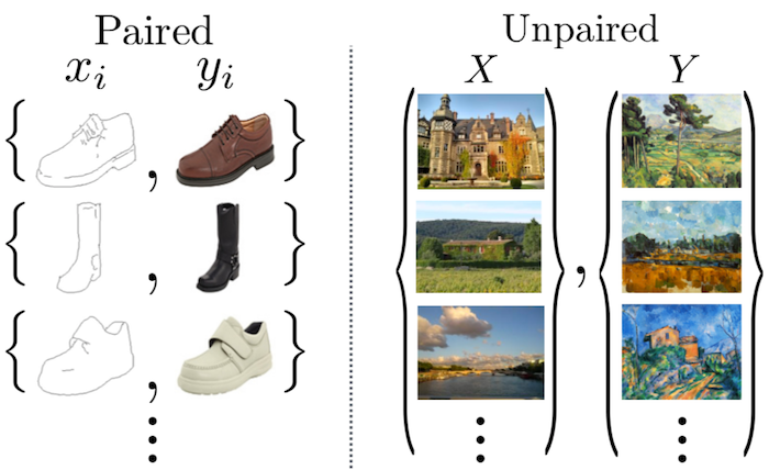
Well, the image below summarizes it well. CycleGAN performs unpaired image to image translation. That means the images we’re training on don’t have to represent the same thing.

It would be (relatively) easy to DaVinci-ify images if we had a large collection of [Math Processing Error](image, painting of image by da Vinci) pairs.
Unfortunately, the dude didn’t get around to completing too many paintings.
CycleGAN, however, trains on unpaired data. So we don’t need two images of the same thing.
On the other hand, we could use style transfer. But that would just extract the style of one particular image and transfer it to another image, meaning we can’t translate from say, horses to zebras.
CycleGAN, however, learns a mapping from one domain of images to another. So we train it on say, the set of all Monet paintings.

The method they use is quite elegant. CycleGAN consists of two generators, [Math Processing Error]G, and [Math Processing Error]F, and two discriminators, [Math Processing Error]DX and [Math Processing Error]DY.
[Math Processing Error]G takes in an image from [Math Processing Error]X and tries to map it to some image in [Math Processing Error]Y. The discriminator [Math Processing Error]DY predicts whether an image was generated by [Math Processing Error]G or was actually in [Math Processing Error]Y.
Similarly, [Math Processing Error]F takes in an image from [Math Processing Error]Yand tries to map it to some image in [Math Processing Error]X, And the discriminator [Math Processing Error]DX predicts whether an image was generated by [Math Processing Error]F or was actually in [Math Processing Error]X.
All four networks are trained in the usual GAN way until we’re left with powerful generators [Math Processing Error]G and [Math Processing Error]F, which can perform the image-to-image translation task well enough to fool [Math Processing Error]DY and [Math Processing Error]DX respectively.
This type of adversarial loss sounds like a good idea. But it isn’t enough. To further improve performance, CycleGAN uses another metric, cycle consistency loss.
Think about the properties of a good translator in general. One of them is that when you translate back and forth, you should get the same thing again.
CycleGAN implements this idea in a clever way. It forces the network to obey these constraints:
[Math Processing Error]F(G(x))≈x,x∈X
[Math Processing Error]G(F(y))≈y,y∈Y
Visually, cycle consistency looks like this:

The overall loss function is constructed in a way that penalizes the networks for not conforming to the above properties. I’m not going to write out the loss function here because that would spoil the way it comes together in the paper.
Ok, now before this becomes a Dragon-ball Z filler fest, let’s get back to our main quest of finding better GAN architectures.
CoGAN: Coupled Generative Adversarial Networks

Image from paper
Do you know what’s better than one GAN? Two GANs!
CoGAN (which stands for “coupled generative adversarial networks,” not to be confused with CGAN, which stands for conditional generative adversarial networks) does just that. It trains a “couple” of GANs rather than a single one.
Of course, GAN researchers just can’t stop making those cop and counterfeiter game theory analogies. So here’s the idea behind CoGAN, in the authors’ own words:
In the game, there are two teams, and each team has two players. The generative models form a team and work together for synthesizing a pair of images in two different domains for confusing the discriminative models. The discriminative models try to differentiate images drawn from the training data distribution in the respective domains from those drawn from the respective generative models. The collaboration between the players in the same team is established from the weight-sharing constraint.
Ok, so having a GAN multiplayer LAN party competition sounds nice and all, but how do you actually make it work?
It turns out it isn’t too complicated. Just make the networks use the exact sameweights for some of the layers.

In my not very humble opinion, the coolest thing about CoGAN isn’t the improved image generation quality or the fact you can train on multiple image domains.
It’s the fact that you get two images for the price of one-and-a-half.
Since we’re sharing some of the weights, a CoGAN would have fewer parameters (and hence would save more memory, compute, and storage) than two individual GANs.
It’s a subtle technique that’s “out-of-fashion” and that some of the newer GANs that we see today don't use.
But one day, I reckon the underdog’s gonna make a comeback.
ProGAN: Progressive growing of Generative Adversarial Networks

Image from paper
- Paper
- Code
- Other great resources: Medium article, Demo video
There are many problems with training GANs. The most important of which is the training instability.
Sometimes, the loss of the GAN can oscillate, as the generator and discriminator undo the learning of the other. Other times, your loss may explode right after the networks converge, and the images start looking horrible.
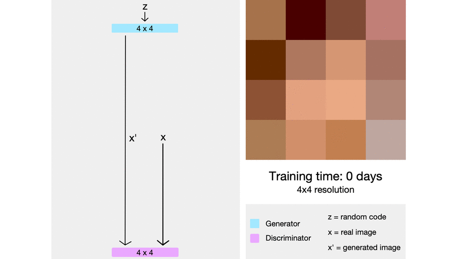
ProGAN (which stands for the progressive growing of generative adversarial networks) is a technique that helps stabilize GAN training by incrementally increasing the resolution of the generated image.
The intuition here is that it’s easier to generate a 4x4 image than it is to generate a 1024x1024 image. Also, it’s easier to map a 16x16 image to a 32x32 image than it is to map a 2x2 image to a 32x32 image.
So ProGAN first trains a 4x4 generator and a 4x4 discriminator and adds layers that correspond to higher resolutions later in the training process. This animation sums up what I’m describing:

WGAN: Wasserstein Generative Adversarial Networks

Image from paper
- Paper
- Code
- Other great resources: DFL Curriculum, Blog post, Another blog post, Medium article
This paper is perhaps the most theoretical/mathematical one on this list. The authors stuffed in a truckload of proofs, corollaries, another mathematical lingo into it. So if Integral probability metrics and Lipschitz continuity aren’t your things, I wouldn’t spend too much time on this one.

In short, WGAN (the ‘W’ stands for Wasserstein) proposes a new cost function that some nice properties that are all the rage for pure mathematicians and statisticians.
Here is the old version of the GAN minimax optimization game:
[Math Processing Error]minGmaxDEx∼pdata(x)[logD(x)]+Ez∼pgenerated(z)[1−logD(G(z))]
And here is the new one that WGAN uses:
[Math Processing Error]minGmaxDEx∼pdata(x)[D(x)]−Ez∼pgenerated(z)[D(G(z))]
For the most part, that’s all you need to know to use WGAN in practice.
Just chuck out the old cost function, which approximates a statistical quantity called the Jensen-Shannon divergence, and slide in the new one, which approximates a statistical quantity called the 1-Wasserstein distance.
Here’s why that’s a big deal:

Image from paper
However, if you’re interested, what follows is a quick review of the mathematical details, which is the very reason that the WGAN paper was so highly acclaimed.
The original GAN paper showed that when the discriminator is optimal, the generator is updated in such a way to minimize the Jensen-Shannon divergence.
If you’re not familiar with it, the Jensen-Shannon divergence is a way of measuring how different two probability distributions are. The larger the JSD, the more “different” the two distributions are, and vice versa. You compute it like this:
[Math Processing Error]JSD(P||Q)=KL(P||P+Q2)+KL(Q||P+Q2)
[Math Processing Error]KL(A||B)=∫−∞∞a(x)loga(x)b(x)dx
However, is minimizing the JSD the best thing to do?
The authors of the WGAN paper thought that it’s probably not. For a particular reason — When the two distributions don’t overlap at all, you can show that the value of the JSD stays at a constant value of [Math Processing Error]2log2
A function that has has a constant value has a gradient equal to zero, and a zero gradient is bad because it means that the generator learns absolutely nothing.
The alternate distance metric proposed by the WGAN authors is the 1-Wasserstein distance, sometimes called the earth mover distance.

Image from paper
It gets the name “earth mover distance” because of an analogy. Imagine that one of the two distributions is a pile of earth, and the other is a pit.
The earth mover distance measures the cost of transporting the pile of earth to the pit, assuming that you’re transporting the mud, sand, dirt, etc., as efficiently as possible. Here, “cost” is considered to be [Math Processing Error]distance between point×amount of earth moved.
Concretely (no pun intended), the earth mover distance between two distributions can be written as:
[Math Processing Error]EMD(Pr,Pθ)=infγ∈Π,∑x,y‖x−y‖γ(x,y)=infγ∈Π E(x,y)∼γ‖x−y‖
Where [Math Processing Error]inf is the infinimum (minimum), [Math Processing Error]x and [Math Processing Error]y are points on the two distributions, and [Math Processing Error]γ is the optimal transport plan.
Unfortunately, computing this is intractable. So instead, we compute something totally different:
[Math Processing Error]EMD(Pr,Pθ)=sup‖f‖L≤1 Ex∼Prf(x)−Ex∼Pθf(x)
The connection between these two equations certainly doesn’t seem evident at first, but through some fancy math called the Kantorovich-Rubenstein duality (try saying that three times fast), you can show that these formulas for the Wasserstein/earth mover distance are trying to calculate the same thing.
If you weren't able to follow along with some of the heavyweight math in the paper and blog posts that I’ve linked to, don’t worry about it too much. Most of the work on WGAN is about providing a complex (read rigorous) justification for an admittedly simple idea.
SAGAN: Self-Attention Generative Adversarial Networks

Image from paper
- Paper
- Code
- Other great resources: Blog post, Medium article
Since GANs use transposed convolutions to “scan” feature maps, they only have access to nearby information.
Using transposed convolutions alone is like painting a picture while only looking at the canvas region within a small radius of your paintbrush.
Even the greatest of artists, who manage to perfect the most exceptional and intricate details, need to take a step back and look at the big picture.
SAGAN (expanded as “self-attention generative adversarial network”) uses the self-attention mechanism that has become extremely popular in recent years thanks to the transformer architecture.
Self-attention allows the generator to take a step back and look at the “big picture.”
BigGAN

- Paper
- Code
- Other great resources: Two-minute papers video, Gradient.pub post, Medium article
After four long years, DeepMind decided to do with GANs what nobody else had attempted before. They used a mystic technique of deep learning so powerful that it made the most technically advanced models quiver in fear as it overtook everything on the state of the art leaderboards with plenty left to spare.
I present to you BigGAN, the GAN that does absolutely nothing (but is run a bunch of TPU clusters, yet somehow deserves to be on this list).

Jokes apart, the DeepMind team did accomplish a lot with BigGAN. Apart from getting all the eyeballs with the realistic imagery, BigGAN showed us some very detailed results of training GANs at large scales.
The team behind BigGAN introduced a variety of techniques to combat the instability of training GANs on huge batch sizes across many machines.
To start with, DeepMind used SAGAN as a baseline and tacked on a feature called spectral normalization.
From there, they scaled the batch size by 50%, width (number of channels) by 20%. Initially, increasing the number of layers didn’t seem to help.
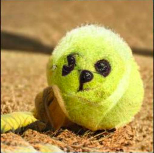
After a few other single digit percentage improvements, the authors use a “truncation trick” to improve the quality of the sampled image.
While BigGAN samples its latent vector from [Math Processing Error]z N(0,I) during training, it resamples the latent vector if it falls outside a given range when generating images.
The range is a hyperparameter, represented by [Math Processing Error]ψ. A smaller [Math Processing Error]ψ tightens the range, which increases sample fidelity at the cost of variety.
So what do all of these intricate tuning effort lead to? Well, some call it dogball:

BigGAN also shows that training GANs at a larger scale can have its own set of problems. Notably, training seems to scale well by increasing parameters like batch size and width, but for some reason, collapses at the very end.
If analyzing singular values to understand this instability sounds interesting to you, check out the paper, because you'll find a lot it there.
Finally, the authors also train BigGAN on a new dataset called JFT-300, which is an ImageNet-like dataset which has, you guessed it, 300 million images. They showed that BigGAN perform better on this dataset, suggesting that more massive datasets might be the way to go for GANs
After the first version of the paper was released, the authors revisited BigGAN a few months later. Remember how I said that increasing the number of layers didn’t work? Turns out that was due to a poor architectural choice.
Instead of just cramming more layers onto the model, the team experimented and found that using a ResNet bottleneck is the way to go.
With all of the above tweaks, scaling, and careful experimentation, the top of the line BigGAN completely obliterates the previous state of the art Inception score of 52.52 with a whopping score of 152.8.
If that isn’t progress, I don’t know what is.
StyleGAN: Style-based Generative Adversarial Networks

Image from paper
- Paper
- Code
- Other great resources: thispersondoesnotexist, Blog post, Another blog post, Technical summary article
StyleGAN (short for well, style generative adversarial network?) is a development from Nvidia research that is mostly orthogonal to the more traditional GAN research, which focuses on loss functions, stabilization, architectures, etc.
Having a world-class face generator that can fool most humans on planet earth is pointless if you want to generate images of cars.
So instead of focusing on creating more realistic images, StyleGAN improves a GANs capability to have fine control over the image that’s generated.
As I mentioned, StyleGAN doesn’t develop on architectures and loss functions. Instead, is a suite of techniques that can be used with any GAN to allow you to do all sorts of cool things like mix images, vary details at multiple levels, and perform a more advanced version of style transfer.
In other words, StyleGAN is like a photoshop plugin, while most GAN developments are a new version of photoshop.
To achieve this level of image style control, StyleGAN employs existing techniques like Adaptive instance normalization, a latent vector mapping network, and a constant learned input.
It’s hard to describe StyleGAN any further without getting into the details, so if you’re interested, check out my article where I show how to generate Game of Thrones characters using StyleGAN. I have a detailed explanation of all the techniques, with a lot of cool results along the way.
Conclusion
Wow, you made it to the end. Congratulation! You're all caught up on the latest breakthroughs in the highly academic domain of creating fake profile pics.
But before you slump onto your couch and begin your endless scroll of your Twitter feed, take a moment to look at how far you've come:

What's next?! Unexplored regions!
After climbing the mountains of ProGAN and StyleGAN, and voyaging across the computational sea to arrive at the vast fields of BigGAN, it's easy to get lost around these parts.
But zoom in. Take a closer look. Do you see that show-shaped green patch of land? The red delta in the north?
Those are the regions unexplored. The breakthroughs waiting to be made. They can all be yours if you choose to take the leap of faith.
Farewell, my friend, there are yet more seas to sail.
Epilogue: Some Interesting Modern Research
Thanks for reading this article. By now, If you've followed all the resources I shared, you should have a solid understanding of some of the most important breakthroughs in GAN technology.
But undoubtedly, there will be more. Keeping up with research will be tough, but it's not impossible. I'd recommend that you try to stick to newer papers since they are likely to produce the best results in your projects.
To get you started, here are a few bleeding-edge (as of May 2019) research projects:
- You've probably heard of DeOldify by now. If not, jump here! But there's been a recent update to it that introduces a new training technique called NoGAN. You can check out the details in their blog and code.
- If you don't have Google-level amounts of data, it can be challenging to replicate the BigGAN results from scratch. There's now an ICML 2019 paperthat proposes to train a BigGAN quality model with fewer labels.
- Of course, GANs aren't the only deep learning based technique for image generation. Recently, OpenAI unveiled a completely new model called the sparse transformer that leverages the transformer architecture for image generation. As usual, they released a paper, blog, and code.
- Oh, and this isn't new research or anything, but you should listen to the origin story of GANs:
- Nvidia has this really cool project called GauGAN which can turn your child's scribblings into photorealistic masterpieces. This is truly something that you need to experience to understand. So play around with the demo first, then read their blog and paper.
- Have you ever wondered how to "debug" a GAN? There's now an ICLR 2019 paper that proposes a promising solution.
- Despite how cool I made GANs look, there's plenty of work to be done. There's an excellent distill article that summarizes some of the unsolved problems.
- It looks like someone has found another type of real-world application for GANs.
Apparently, GANs are used to create fake profile pictures on LinkedIn for international industrial espionage. https://t.co/IFYJwb30cw
— Yann LeCun (@ylecun) June 13, 2019
FloydHub Call for AI writers
Want to write amazing articles like Ajay and play your role in the long road to Artificial General Intelligence? We are looking for passionate writers, to build the world's best blog for practical applications of groundbreaking A.I. techniques. FloydHub has a large reach within the AI community and with your help, we can inspire the next wave of AI. Apply now and join the crew!
About Ajay Uppili Arasanipalai
Ajay is a deep learning enthusiast and student at the University of Illinois at Urbana-Champaign. Ajay is a FloydHub AI Writer (you can read his previous FloydHub article here). He writes technical articles for blogs like FloydHub, Freecodecamp, HackerNoon, and his own blog, Elliptigon. You can connect with Ajay via LinkedIn, Twitter, Medium, Reddit, and GitHub.