Machine learning and Data Mining - Association Analysis with Python

Recently I've been working with recommender systems and association analysis.  This last one, specially, is one of the most used machine learning algorithms to extract from large datasets hidden relationships. 

The famous example related to the study of association analysis is the history of the baby diapers and beers. This history reports that a certain grocery store in the Midwest of the United States increased their beers sells by putting them near where the stippers were placed. In fact, what happened is that the association rules  pointed out that men bought diapers and beers on Thursdays. So the store could have profited by placing those products together, which would increase the sales.

Association analysis is the task of finding interesting relationships in large data sets. There hidden relationships are then expressed as a collection of association rules and frequent item sets.  Frequent item sets are simply a collection of items that frequently occur together.  And association rules suggest a strong relationship that exists between two items.  Let's  illustrate these two concepts with an example.

A list of transactions from a grocery store is shown in the figure above. Frequent items are a list of items that commonly appear together.  One example is {wine, diapers, soy milk}.  From the data set we can also find an association rule such as diapers -> wine.  This means that if someone buys diapers, there is a good chance they will buy wine. With the frequent item sets and association rules retailers have a much better understanding of their customers.  Although common examples of association rulea are from the retail industry, it can be applied to a number of other categories, such as web site traffic, medicine, etc.

How do we define these so called relationships ? Who defines what is interesting ?  When we are looking for frequent item sets or association rules, we must look two parameters that defines its relevance.  The support of an itemset, which is defined as the percentage of the data set which containts this itemset. From the figure above the support of {soy milk} is 4/5. The support of {soy milk, diapers } is 3/5 because of the five transactions, three contained both soy milk and diapers. Support applies  to an itemset, so we can define a minimum support and only get the itemsets that meet that minimum support. And the cofidence which is defined for an association rule like diapers->wine. The confidence for this rule is defined as support({ diapers, wine})/ support(diapers).  From the figure above, support of {diapers, wine} is 3/5. The support for diapers is 4/5, so the confidence for diapers -> wine  is: 3/4 = 0.75.  That means in 75% of the items in our data set containing diapers our rule is correct.

The support and confidence are ways we can quantify the success of our association analysis. Let's assume we wanted to find all sets of items with a support greater than 0.8. How would we do that ?  We could generate a list of every combination of items then go and count how frequent that occurs. But this is extremely slow when we have thousands of items for sale. In the next section, we will analyze the Apriori principle which address this problem and reduces the number of calculations we need to do to learn association rules.

To sum up, one example of rule extracted from associatio analysis:

"If the client bought the product A1 and the product A4, so he also bought the product A6 in 74% of the cases. This rule applies on 20% of the studied cases."

The first parameter is the support, that is, the percentage of cases that the product A1 appears in the frequent item sets.  In the rule above, the value 20% points the support, which reports that the rule is applied on 20% of the studied cases.  The second parameter is the confidence, which tells the percentage of occurrences of the rule.  So the value 74% represents the confidence,  where in the 20% of the rules where products A1 and A4 are found, 74% of them we also can find the product A6.

Apriori Algorithm

Let's assume that we are running a market store with a very limited selection. We are interested in finding out which items were purchased together. We have only four items: item0, item1, item2 and item3. What are all the possible combinations that can be purchased ? We can have one item, say item0 alone, or two items, or threee items, or all of the items together. If someone purchased two of item0 and four of item2, we don't care. We are concerned only that they purchased one or more of an item.

A diagram showing all possible combinations of the items is shown in the figure above.  To make easier to interpret, we only use the item number such as 0 instead of item0.  The first set is a big Ø, which means the null set or a set containing no items. Lines connecting item sets indicate that two or more sets can be combined to form a larger set.

Remember that our goal is to find sets of items that are purchased together frequently. The support of a set counted the percentage of transactions that contained that set. How do we calculate this support for a given set, say {0,3}? Well. we go through every transaction and ask, ”Did this transaction contain 0 and 3?” If the transaction did contain both those items, we increment the total. After scanning all of our data, we divide the total by the number of transactions and we have our support. This result is for only one set: {0,3}. We will have to do this many times to get the support for every possible set. We can count the sets in Figure below and see that for four items, we have to go over the data 15 times. This number gets large quickly. A data set that contains N possible items can generate 2N-1 possible itemsets. Stores selling 10,000 or more items are not uncommon. Even a store selling 100 items can generate 1.26*1030 possible itemsets. This would take a very, very long time to compute on a modern computer.

To reduce the time needed to compute this value, researchers identified something called the Apriori principle. The Apriori principle helps us reduce the number of possible interesting itemsets. The Apriori principle is: if an itemset is frequent, then all of its subsets are frequent. In Figure below this means that if {0,1} is frequent then {0} and {1} have to be frequent. This rule as it is doesn’t really help us, but if we turn it inside out it will help us. The rule turned around reads: if an itemset is infrequent then its supersets are also infrequent, as shown in Figure  below.

As you can observe, the shaded itemset {2,3} is known to be infrequent. From this knowledge, we know that itemsets {0,2,3}, {1,2,3}, and {0,1,2,3} are also infrequent. This tells us that once we have computed the support of {2,3}, we don’t have to compute the support of {0,2,3}, {1,2,3}, and {0,1,2,3} because we know they won’t meet our requirements. Using this principle, we can halt the exponential growth of itemsets and in a reasonable amount of time compute a list of frequent item sets.

Finding frequent item sets

Now let's go through the Apriori algorithm.  We first need to find the frequent itemsets, then we can find association rules. The Apriori algorithm needs a minimum support level as an input and a data set. The algorithm will generate a list of all candidate itemsets with one item. The transaction data set will then be scanned to see which sets meet the minimum support level. Sets that do not meet the minimum support level will get tossed out. The remaining sets are then combined to make itemsets with two elements. Again, the transaction data set will be scanned and itemsets not meeting the minimum support level will get tossed. This procedure is repeated until all sets are tossed out.

We will use Python with Scipy and Numpy to implement the algorithm. The pseudocode for the Apriori Algorithm would look like this:

While the number of items in the set is greater than 0:

               Create a list of candidate itemsets of length k 

              Scan the dataset to see if each itemset is frequent

             Keep frequent itemsets to create itemsets of length k+1

The code in Python is shown below:

12345678910111213141516171819202122232425262728293031323334353637383940414243444546474849505152535455565758596061626364656667686970

#-*- coding:utf-8 - *-     def load_dataset(): "Load the sample dataset." return [[1, 3, 4], [2, 3, 5], [1, 2, 3, 5], [2, 5]]     def createC1(dataset): "Create a list of candidate item sets of size one." c1 = [] for transaction in dataset: for item in transaction: if not [item] in c1: c1.append([item]) c1.sort() #frozenset because it will be a ket of a dictionary. return map(frozenset, c1)     def scanD(dataset, candidates, min_support): "Returns all candidates that meets a minimum support level" sscnt = {} for tid in dataset: for can in candidates: if can.issubset(tid): sscnt.setdefault(can, 0) sscnt[can] += 1   num_items = float(len(dataset)) retlist = [] support_data = {} for key in sscnt: support = sscnt[key] / num_items if support >= min_support: retlist.insert(0, key) support_data[key] = support return retlist, support_data     def aprioriGen(freq_sets, k): "Generate the joint transactions from candidate sets" retList = [] lenLk = len(freq_sets) for i in range(lenLk): for j in range(i + 1, lenLk): L1 = list(freq_sets[i])[:k - 2] L2 = list(freq_sets[j])[:k - 2] L1.sort() L2.sort() if L1 == L2: retList.append(freq_sets[i] | freq_sets[j]) return retList     def apriori(dataset, minsupport=0.5): "Generate a list of candidate item sets" C1 = createC1(dataset) D = map(set, dataset) L1, support_data = scanD(D, C1, minsupport) L = [L1] k = 2 while (len(L[k - 2]) > 0): Ck = aprioriGen(L[k - 2], k) Lk, supK = scanD(D, Ck, minsupport) support_data.update(supK) L.append(Lk) k += 1   return L, support_data

view rawApriori.py hosted with ❤ by GitHub

The source is docummented so  you can easily understand all the rules generation process.

Let's see in action ?!

First, we created our first candidate item set C1. C1 contains a list of all items in frozenset. After we created D, which is just a dataset in the form of list of sets (set is a list of unique elements).  With everything in set form we removed items that didn't meet our minimum support. So in our example 0.5 was the minimum support level chosen.  The result is represented by the list L1 and support_data. These four items that make our list L1 are the sets that occur in at least 50% of all transactions. Item 4 didn't make the minimum support level, so it's not a part of L1. By removing it, we have removed more work we needed to do when wen find the list of two-item-sets. Remember our pruned tree above?!

Two more functions now were used: apriori() and aprioriGen(). In apriori() given a data set and a support level, it will generate a list of candidate itemsets. AprioriGen() is responsible for generate the next list of candidate itemsets and scanD throw out itemsets that don't meet the minimum support levels. See the result of aprioriGen() it generates six unique two-item-sets.  If we run it with our apriori function we will check that L contains some lists of frequent itemsets that met a minimum support of 0.5.  The variable support_data is just a dictionary with the support values of our itemsets.  We don't care about those values now, but it will be useful in the next section.   We have now which items occur in 50% of all transactions and we can begin to draw conclusions from this.  In the next section we will generate association rules to try to get an if-then understanding of the data.

Mining association rules from frequent item sets

We just saw how we can find frequent itemsets with Apriori Algorithm. Now we have to find the association rules. To find them, we first start with a frequent itemset.  The set of items is unique, but we can check if there is anything else we can get out of these items. One item or one set of items can imply another item. From the example above, if we have a frequent itemset: {soy milk lettuce}, one example of an association rule is: soy milk -> lettuce.  This means if someone purchases soy and milk, then there is a statistically significant chance that he will purchase lettuce. Of course this is not always true, that is, just because soy milk -> lettuce is statistically significant, it does not mean that lettuce -> soy milk will be statistically significant.

We showed the support level as one measurement for quantifying the frequency of an itemset. We also have one for association rules. This measurement is called the confidence. The confidence for a rule P-> H is defined as: support (P|H)/support(P).  Remember that the | symbol is the set union. P|H means all the items in set P or in set H.  We already have the support values for all frequent itemsets provided in apriori function, remember ?  Now, to calculate the confidence, all we have todo is call up those support values and do one divide.

From one frequent itemset, how many association rules can we have ?  If you see the figure below, it shows all the different possible associations rules from the itemset {0, 1, 2, 3}. To find relevant rulese, we simply generate a list of possible rules, then test the confidence of each rule. If the confidence does not meet our minimum requirement, then we throw out the rule.

Usually we don't this. Imagine the number of rules if we have a itemset of 10 items, it would be huge. As we did with Apriori Algorithm we can also reduce the number of rules that we need to test. If the rule does not meet the minimum confidence requirement, then subsets of that rule also will not meet the minimum. So assuming that the rule 0,1,2 -> 3 does not meet the minimum confidence, so any rules where is subset of 0,1,2 ->3 will also not meet the minimum confidence.

By creating a list of sets with one item on the right hand size, testing them and merging the remaining rulese, we can create a list of rules of two items and do this recursively. Let's see the code below:

123456789101112131415161718192021222324252627282930313233343536373839

def generateRules(L, support_data, min_confidence=0.7): """Create the association rules L: list of frequent item sets support_data: support data for those itemsets min_confidence: minimum confidence threshold """ rules = [] for i in range(1, len(L)): for freqSet in L[i]: H1 = [frozenset([item]) for item in freqSet] print "freqSet", freqSet, 'H1', H1 if (i > 1): rules_from_conseq(freqSet, H1, support_data, rules, min_confidence) else: calc_confidence(freqSet, H1, support_data, rules, min_confidence) return rules     def calc_confidence(freqSet, H, support_data, rules, min_confidence=0.7): "Evaluate the rule generated" pruned_H = [] for conseq in H: conf = support_data[freqSet] / support_data[freqSet - conseq] if conf >= min_confidence: print freqSet - conseq, '--->', conseq, 'conf:', conf rules.append((freqSet - conseq, conseq, conf)) pruned_H.append(conseq) return pruned_H     def rules_from_conseq(freqSet, H, support_data, rules, min_confidence=0.7): "Generate a set of candidate rules" m = len(H[0]) if (len(freqSet) > (m + 1)): Hmp1 = aprioriGen(H, m + 1) Hmp1 = calc_confidence(freqSet, Hmp1, support_data, rules, min_confidence) if len(Hmp1) > 1: rules_from_conseq(freqSet, Hmp1, support_data, rules, min_confidence)

view rawApriori_rules.py hosted with ❤ by GitHub

Let's see in action:

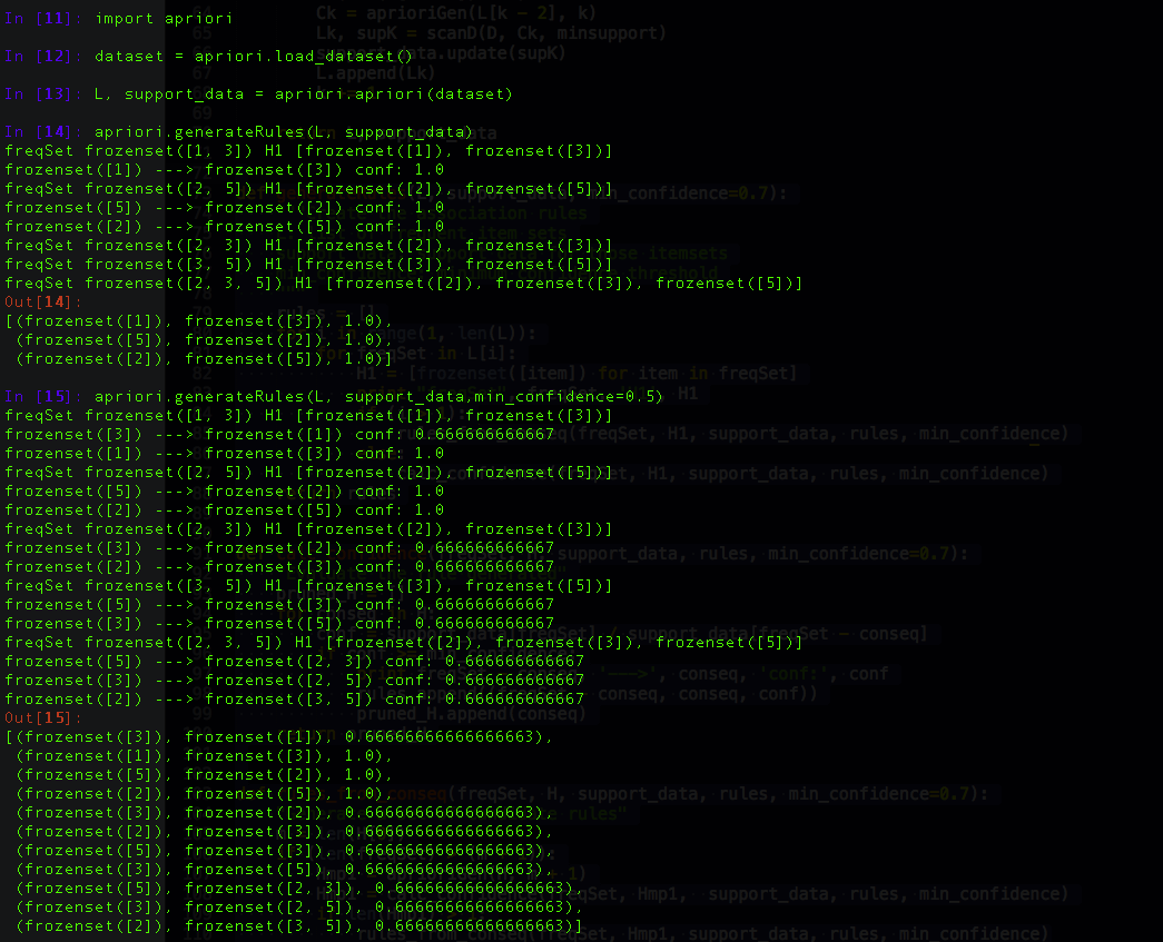
As you may seen in the fist call, it gives us three rules: {1} -> {3} , {5} -> {2} and {2} -> {5}. It is interesting to see the rules with 2 and 5 can be flipped around, but not the rule with 1 and 3. If we lower the confidencer threshold to 0.5, we may see more rules.  Let's go now to a real-life dataset and see how it does work.

Courses  at Atepassar.com

It's time to see these tools on a real life dataset. What can we use ?  I love educational data, so let's see an example using the Atepassar social network data. Atepassar is a popular social-learning environment where people can organzie the studies for public exams in order to get a civil job. I work there as Chief Scientist!

The data set provided can give us some interesting insights about the profiles of the users who buys on-line courses at Atepassar. So we will use the apriori() and generateRules() functions to find interesting information in the transactions.

So let's get started.  First I will create a transaction database and then generate the list of frequent itemsets and association rules.

Collect Dataset from Atepassar.

So let's get started.  First I will create a transaction database and then generate the list of frequent itemsets and association rules.

I have encoded some information related to our transactions, for example, the client's user profile such as state, gender and degree. I also extracted the bought courses and the category of the course such as 'national', 'regional', 'state' or 'local'.

This give us important hypothesis to test like "Male people buy more preparation courses for national exams?", "People from Sao Paulo tends to buy more for state exams ?" or even if male people graduated buys courses for 'local' exams ?"  Those are some examples of explanations that we may get with association analysis.

After loading my dataset we can see inside each transaction:

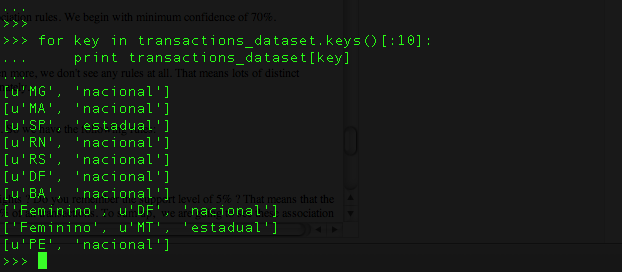
Let's see one of them in order to explain it:

So one transaction is composed by a woman who bought a preparation course for a national exam (Brazilian exam) and lives at Distrito Federal (DF).

Now,  let's use our Apriori algorithm. But first let's make a list of all the transactions. We will throw out the keys, which are the usernames. We are not interested in that.  What we are interested is the items and associations among them.  Now let's going to mine the frequent itemsets and association rules.

Applying the Apriori algorithm developed earlier,  and use support settings of 5%, we may see several of frequent itemsets. 

Now let's try to generate the association rules. We begin with minimum confidence of 70%.  

If we increase the confidence even more, we don't see any rules at all. That means lots of distinct transactions or  small amount of data unfortunately.

I will be with confidence of 70%. So we have the following rules:

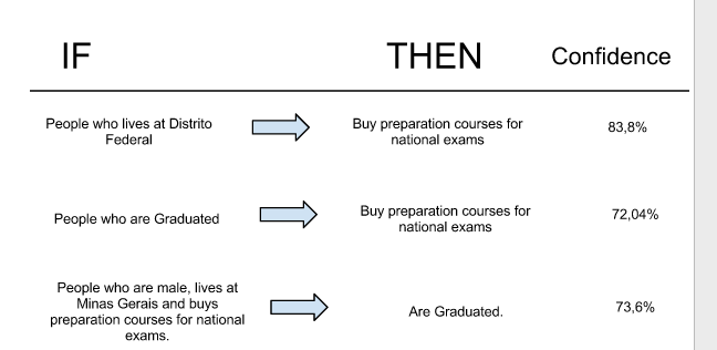
What can we say about those insights ? Do you remember the support level of 5% ? That means that the rules above show up in at least 5% of all transactions. To sum up,  we are going to see these association rules in at least 5% of the transactions, and in the case of  DF --> Nacional, this rule is right 83,8% of the time.  People from Brasilia really purchase for better positions in the government,  or even get the best salaries! 

Conclusions

In this post I presented one of the most traditional tools in data mining to find interesting relationships in a large set of data.  We saw that there are two ways we can quantify the relationships: using frequent itemsets, which shows items that commonly appear in the data together. And the second one are the association rules which imply an if -> t hen relationship between items.

But wait,  before start using it at your dataset, I have to give sou some warnings.  Finding different combinations of items can be a very consuming task and expensive in terms of computer proccessing.  So you will need more intelligent approaches to find frequent itemsets in a small amount time.  Apriori is one approach that tries to reduce the number of sets that are chacked against the dataset. With Support measure and Confidence we can combine both to generate association rules. 

The main problem of Apriori Algorithm is it requires to scan over the dataset each time we increase the length of our frequent itemsets. Imagine with a huge dataset, it can slow down the speed of finding frequent itemsets.  Alternative techniques for this issue is the FP-Growth algorithm, for example. It only needs to go over the dataset twice, which can led to a better performance.

The code in Python is shown here.